3. Multiple Object Classification and Tracking

3.1. Multiple Object Classification

Multiple object detection and classification is required for tracking humans and vehicles. Object detection is the process of identifying multiple objects of the interest classes and localizing these identified objects with their bounding box information. Multiple object detection can be broadly divided into traditional and deep learning approaches. In the recent years deep learning approaches have surpassed the traditional approaches because of the huge labelled training data and GPU processing.

Deep learning based Convolutional neural networks for multiple object detection can be categorized as (a) Region based (two-stage) detectors, (b) Single stage detectors and (c) Keypoints based detectors. Single stage detctors are not as accurate as Keypoints based and Region based detectors, but have comparative accuracy and very high running speeds and thus much more useful in real time applications. In rhis work we make use of single stage object detector called Yolov3, which can run in real time.

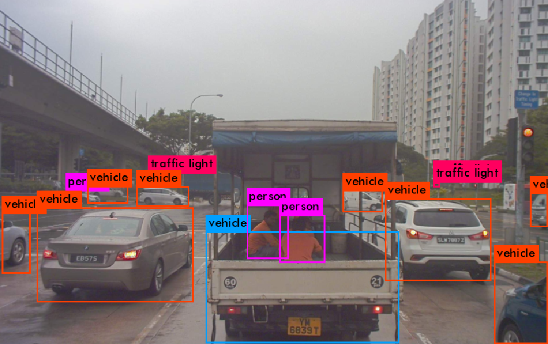
When compared to the previous Point Grey stereo system, with the new camera system colour information is being made available. Therefore, we now can use the weight files for classification network that has been trained on large datasets that have shown higher accuracy in COCO train & val set. In this work we calssify and detect objects in seven object classes such as;

• person

• vehicle

• bicycle

• traffic light

• parking meter

• bench

• stop sign

These object detections are then associated with the 3D information from stereo and then used in tracking algorithm. Each object is associated with below information;

• object class

• object bounding box (x,y,width,height)

• detection confidence

• X,Y,Z to the object center with reference to the left camera center (local window)

• width and height in meters

Detection result from Yolov3 is as below.

3.2. Multiple Object Tracking

Tracking research can broadly be divided in to multiple Object Tracking (MOT) and single object tracking. While MOT assumes object detection as prior knowledge, the latter tries to localize and track an unknown object that has only been described by the localization information at the first frame. In this work, we propose a method to address MOT by defining a dissimilarity measure based on object motion, appearance, structure and size. We follow tracking-by-detection framework.

The proposed tracking method mainly consists of three major components, (a) Dissimilarity Cost Computation, (b) Track Match and Update and (c) Tracking False Negatives for Stable Tracks, which are discussed in detail in this section. Since we are following the tracking by detection framework, for the proposed tracking method we assume that at every frame a set of object bounding boxes along with object class and detection confidence is available. The overall tracking process is presented as a flow chart in Fig. 3.4.

Fig. 3.4 Flow chart of the proposed tracking framework, where \(bb_{i,det}\) is the bounding box of the \(i^{th}\) detection, \(LBPH\) stands for Linear Binary Pattern Histogram and \(dis(i,j)\) is the dissimilarity cost between \(i^{th}\) object detected in the current frame with the \(j^{th}\) object in the track list.

3.2.1. Dissimilarity Cost Computation

Dissimilarity cost \(dis(i,j)\) between \(i^{th}\) detection in the current frame with the \(j^{th}\) object in the track list is defined as a weighted sum of four distance measures based on appearance distance \(app(i,j)\), structural distance \(str(i,j)\), location difference \(loc(i,j)\) and size difference \(iou(i,j)\) as defined in (3.9).

(3.9)\[\begin{equation} dis(i,j) = w_{app}\cdot app(i,j) + w_{str}\cdot str(i,j) + w_{loc}\cdot loc(i,j) + w_{iou}\cdot iou(i,j) \end{equation}\]

\(w_{app}, w_{str}, w_{loc}\) and \(w_{iou}\) are the weights for the contributions from each of the four distance measures. All four distance measures are defined such that they vary between 0 and 1.

Appearance based Distance

In this work we propose a grid based multiple histogram matching method as an appearance feature. Appearance based distance is measured using the correlation between the colour histograms of the \(i^{th}\) detection and \(j^{th}\) track. Histogram matching is done against a maximum of three colour histograms extracted from the history of the track. In this work we consider the HSV (hue, saturation, value) colour space because it is more robust for illumination changes compared to the RGB (red, green, blue) colour space. Hence we use H and S variants for histogram matching. Furthermore, a grid based structure is used when calculating the histogram for each object bounding box. This results in \(n\) (number of grid cells per bounding box) number of histograms, which is then concatenated to create a single histogram. Since an object can be partially occluded in a given instance, we define an occlusion map for this grid structure to be used when matching histograms to avoid any bias from inaccurate information. Fig. 3.5 visualize an example on the grid structure and the appearance history of a track.

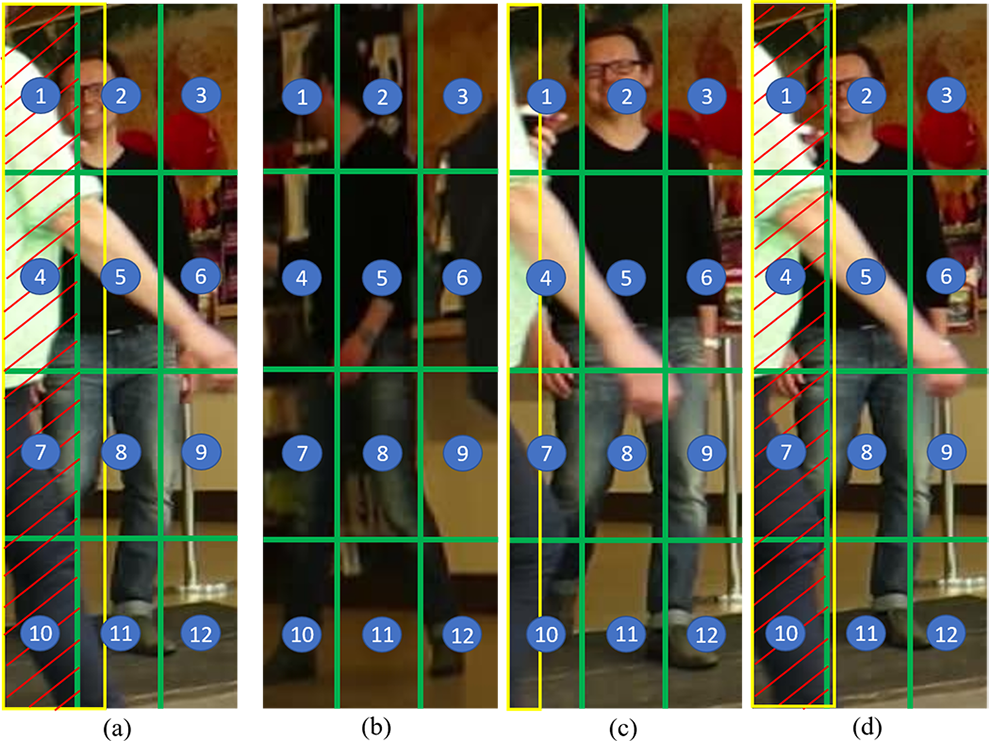
Fig. 3.5 Grid structure and appearance based history of a track. (a) current frame matched detection and (b), (c) and (d) are the visualizations of the three appearance history of the matched track kept in memory. Green boxes indicate the grid structure and shaded area by red lines indicate the occlusion. Yellow colour indicates the bounding box of the object in front of the track. Grid is \(3 \times 4\). \(1^{st}, 4^{th}, 7^{th}\) and \(10^{th}\) grid cells are occluded due to object in front (yellow bounding box) for (a) and (d). \(2^{nd}, 5^{th}, 8^{th}\) and \(11^{th}\) grid cells are considered non-occluded as yellow bounding box does not cover at least 50% of the grid cell area. No grid cell is occluded for (b) and (c). When appearance matching, \(2^{nd}\) grid cell of (a) is compared with $2^{nd}$ grid cells of (b), (c) and (d) and average is taken. \(1^{st}, 4^{th}, 7^{th}\) and \(10^{th}\) grid cells are not considered because it is occluded for (a) and all the remaining grid cells are considered in matching.

Appearance based distance between $i^{th}$ detection and \(j^{th}\) track is defined as in (3.10).

(3.10)\[\begin{equation} app(i,j) = 1.0 - \frac{\sum_{k}\sum_{n}occl(n,i) \cdot occl(n,j)^k \cdot corr(H_{n,i},H_{n,j}^k)}{n\cdot k} \end{equation}\]

where \(k\) is the number of concatenated histograms kept in the memory for each track from its history which can be up to a maximum of three. \(n\) is the number of cells in the grid. The procedure followed in updating histograms for a track. \(occl(n,i)\) and \(occl(n,j)^k\) are the occlusion indicators for the \(n^{th}\) grid cell of the \(i^{th}\) detection and \(n^{th}\) grid cell of the \(j^{th}\) track of the \(k^{th}\) history map, respectively. \(corr(H_{n,i},H_{n,j}^k)\) is the correlation between the histogram of the \(n^{th}\) grid cell of the \(i^{th}\) detection \(H_{n,i}\) and \(n^{th}\) grid cell of the \(j^{th}\) track of the \(k^{th}\) history map \(H_{n,j}^k\). Correlation indicates the similarity between two histograms and output a value between 0 and 1. Hence, we divide the sum of histogram correlations by total number of histograms ($n*k$) and take one minus that as the appearance distance.

(3.11)\[\begin{equation} corr(H_{a},H_{b}) = \frac{\sum_{I}(H_a(I)-\bar{H_a})(H_b(I)-\bar{H_b})}{\sqrt{\sum_{I}(H_a(I)-\bar{H_a})^2\sum_{I}(H_b(I)-\bar{H_b})^2}} \end{equation}\]

where,

(3.12)\[\begin{equation} \bar{H_c} = \frac{1}{N}\sum_{J}H_c(J) \end{equation}\]

in which \(N\) is the total number of bins in the histogram.

Occlusion parameter \(occl\) for each grid cell is either 1 or 0 depending on the level of occlusion for that particular grid cell. Level of occlusion is defined based on the bounding box overlap. If any two or more bounding boxes overlap with each other, the bounding box belonging to the object that has the highest detection confidence is considered to be in front and the overlapping areas with other bounding boxes are considered to be occluded areas for those bounding boxes. Then in a given grid cell, if more than 50% of the pixels are occluded in such a way, the occlusion parameter for that grid cell is set to 0, otherwise set to 1. This is expressed below, where \(M_{n,i}\) is the total number of pixels in the \(n^{th}\) grid cell and \(m_{occl,n,i}\) is the number of pixels occluded in that cell.

(3.13)\[\begin{split}\begin{equation} occl(n,i) = \begin{cases} 1; & if \;m_{occl,n,i}>0.5\times M_{n,i}\\ 0; & otherwise \end{cases} \end{equation}\end{split}\]

Structure based Distance

Linear Binary Pattern (LBP) is a good feature that can capture structural information from an image and is a robust feature for illumination variances. LBP outputs a binary code word for each pixel by comparing pixels values in a 3x3 neighbourhood with the center pixel value. Such example is presented in Fig. 3.6. LBP image is a collection of 8 bit binary code words out of all possible code words (in 3x3 neighbourhood \(2^{9-1}=256\) code words), that can be represented as a histogram. This is known as the LBP Histogram (LPBH).

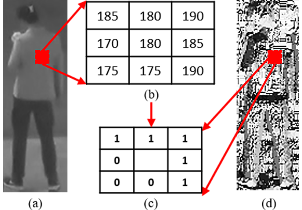
Fig. 3.6 Linear Binary Pattern (LBP). (a) Gray scale image. (b) Zoom-in view of the area of the red box of (a). (c) LBP of (b). (d) LBP of full image (a).

The correlation between two structures in adjacent frames as the structure of an object in not expected to change drastically in adjacent frames of a video. Hence, we use grid based LBPHs to define a distance measure in this tracking task. The same grid structure described in earlier is used here was well. Unlike during the appearance based matching, we only match the concatenated LBPH of the detection with the most recent concatenated LBPH of the track. The structure based distance measure between \(i^{th}\) detection and \(j^{th}\) track, \(str(i,j)\) is as defined below.

(3.14)\[\begin{equation} str(i,j) = 1.0 - \frac{\sum_{n} corr(LBPH_{n,i},LBPH_{n,j})}{n} \end{equation}\]

where \(corr(LBPH_{n,i},LBPH_{n,j})\) is the correlation between the LBPH of the \(n^{th}\) grid cell of the \(i^{th}\) detection \(LBPH_{n,i}\) and \(n^{th}\) grid cell of the \(j^{th}\) track \(LBPH_{n,j}\).

Motion based Distance

When tracking an object in adjacent frames, its motion helps to predict the position of the object in the next frame. We define the difference between the predicted position \(pred(x,y)\) and the measured position \(det(x,y)\) as the motion based distance measure as in (3.15). L2 norm is used. \(x\) and \(y\) are the center positions of the object bounding box expressed in 2D image coordinates. \(n_{dst}\) is the value used to normalize the distance measure.

(3.15)\[\begin{equation} loc(i,j) = \min \Bigg( 1 \; , \; \frac{\| \: det(x,y)-pred(x,y) \: \|_2}{n_{dst}} \Bigg) \end{equation}\]

Predicted position \(pred(x,y)\) is calculated based on the object bounding box information from its track history. The predictions for the bounding box center \((x,y)\), width \(w\) and height \(h\) is generated using a weighted average of it’s previous five frames information. We use five frames because it is large enough to get good average for predictions and small enough not to drift because of old information. We use weights to give a higher weightage to the information from the most recent track assignments in the history. When less than five frames predicted bounding box is the most recent bounding box in the history of the track \(bb_{j}^t\). Width of the most recent bounding box \(w_{bb_{j}^t}\) is used as \(n_{dst}\).

Size based Distance

Size based dissimilarity is calculated based on the object localization information (object bounding box) of each detection compared to the predicted localization information from object track history. Specifically, intersection over union (IoU) between the detection bounding box \(bb_{i,det}\) of the \(i_{th}\) detection and the predicted bounding box \(bb_{j,pred}\) of the \(j_{th}\) track is considered. IoU is inversely proportional to the dissimilarity between two bounding boxes and the IoU will directly provide the similarity value normalized to \(0 - 1\). Therefore, size based dissimilarity is defined as below.

(3.16)\[\begin{equation} iou(i,j)=1-\frac{bb_{i,det} \cap bb_{j,pred}}{bb_{i,det} \cup bb_{j,pred}} \end{equation}\]

IoU is measured considering both the location and size of the bounding boxes in comparison, thus is a good measure of the location similarity of bounding boxes. Predicted bounding box \(bb_{j,pred}\) for the \(j^{th}\) track is as below in(ref{eq:9}), where \(bb_{j}^t\) and \(bb_{j}^p\) is as in (3.17).

(3.17)\[\begin{split}\begin{equation} bb_{j,pred} = \begin{cases} bb_{j}^t; & if \;t<5\\ bb_{j}^p; & otherwise \end{cases} \end{equation}\end{split}\]

3.2.2. Track Match and Update

Once all four dissimilarity measurements are calculated, overall dissimilarity values \(dis(i,j)\) is calculated between each detection in the current frame against each track in the memory. Therefore, this dissimilarity matrix is used in the Hungarian algorithm to assign each of the object detection in the current frame to the best matching track. However, this association is done only if the dissimilarity between the matched detection and track is below a certain threshold \(th_{dis}\), otherwise the detected object is initiated as a new track after tracking for false negatives.

In the detection and track association stage, object information in the list of tracks is updated with the current detection’s localization co-ordinates, LBPHs and detection confidence. Appearance based histograms and occlusion information are updated in a different manner. For each track three most relevant concatenated appearance histogram and occlusion information are stored. Firstly, from the already existing three most relevant concatenated histograms the most occluded one is removed. If the level of occlusion is similar, the oldest concatenated histogram is removed. Then the current matched detection’s concatenated appearance histogram and occlusion information is stored for the track.

3.2.3. Tracking False Negatives for Stable Tracks

One of the applications of a tracking algorithm following tracking-by-detection framework is to identify and maintain the track of an object that goes undetected in some frame/frames (as a result of a false negative of the detection algorithm), of a stable track. In this section we discuss the method we propose to address this challenge.

A track is stable if it has been tracked in at least five previous frames, as it is the number of frames required to predict the next location. After the Hungarian assignment there are three outputs, (a) detection matched with a track, (b) unmatched detection and (c) unmatched track. For each of these unmatched tracks, size based dissimilarity measure is calculated against all the unmatched detections, with the predicted bounding box. If none of the above size based dissimilarity measures, is not less than a threshold \(th_{iou}\) (0.5 is used), we calculate the appearance based dissimilarity with a new detection defined using the predicted bounding box. If the appearance based dissimilarity is less than a threshold (0.6 is used) the predicted bounding box for that track is considered as its current frame match. However, if the predicted bounding box is out of the frame, the corresponding track is immediately marked as an invalid track.

In case of at least one detection has a dissimilarity measure less than \(th_{iou}\), these tracks and detections are considered in Hungarian assignment and matched with each other. Association is done only if the dissimilarity between the matched detection and track is below the same threshold \(th_{iou}\), otherwise the detected object is initiated as a new track.

After updating the track list with the current matched detection data and tracking for false negatives, the track list is updated to invalidate certain tracks which have not being tracked (i.e. matching object not found) for a predefined consecutive number of frames.